Using the Quantlab Python Interface

Overview

All functions available in Quantlab may be called from any Python 3.x environment. This includes:

• The built-in library of financial and mathematical functions

• User-written functions and classes implemented in QLang (saved as library files)

• Compiled C/C++ binaries implemented as QLL Dynamic Link Libraries

• Real-time connections to Bloomberg and Refinitiv

The Python interface is the easiest way to get started with Quantlab programmatically. No compilation, no COM registration – just import ql and go.

Installing the Python Quantlab API

The python folder under the Quantlab root contains version-specific subfolders:

Folder	Python version
py3x-64	Python 3.x, 64-bit (recommended)
py3x-32	Python 3.x, 32-bit
py27-64	Python 2.7, 64-bit (legacy)
py27-32	Python 2.7, 32-bit (legacy)

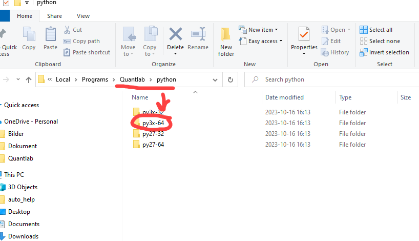
Option 1: System Environment Variable

Add a system variable PYTHONPATH pointing to the corresponding Python version folder. Any time Python is started it will recognize the Quantlab library.

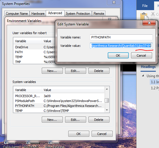
Option 2: Dynamic Path (recommended)

Add the Python path at runtime using sys.path.append(). This works for any user regardless of system environment:

import sys
sys.path.append('C:/Algorithmica/Quantlab/python/py3x-64')
import ql

Once imported, the session loads all library functions set in the ini-file. If instr31.dll is available and a valid ODBC source points to an instrument and curve database, instrument definitions are loaded automatically – the same as starting a Quantlab session.

Note: Loading of the Quantlab function set including your internal ql/qll library files is done automatically every time import ql runs. There is no need to export and register tlb files as with the COM connection.

Python Examples

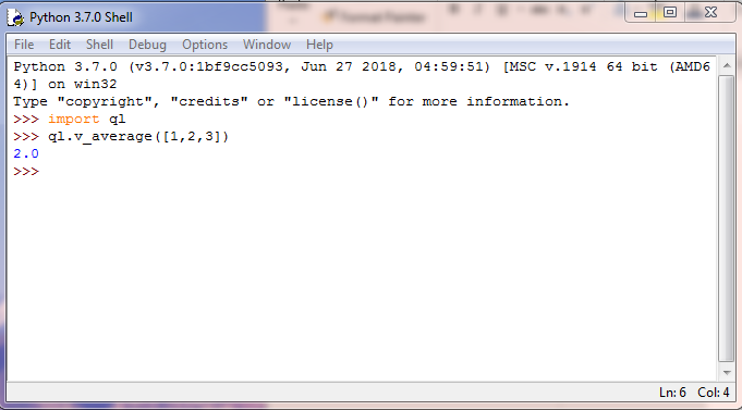
The Quantlab Python API works equally well from the Python IDLE command shell, Jupyter notebooks, and regular Python scripts.

Basic Usage – Python Shell

>>> import ql
>>> ql.v_average([1, 2, 3])
2.0

Yield Curve Plotting with Matplotlib

Plot the government bond yield curve using Quantlab curve construction and matplotlib:

import matplotlib.pyplot as plt
import ql

# Build the discount function once
c = ql.curve("SEKGOVT", ql.today(), "MID")
df = ql.tension_spline_y(c, ql.interpolation(ql.ip_linear(), [1], [0.1]))

# Extract yields at maturities 1Y to 30Y
t = ql.range_vector(1, 30)
s = [df.effective_rate_spot(myt) * 100 for myt in t]

fig, ax = plt.subplots()
ax.plot(t, s)
ax.set(xlabel='Maturity (years)', ylabel='Yield (%)',
       title='Government Bond Yield Curve')
ax.grid()
plt.show()

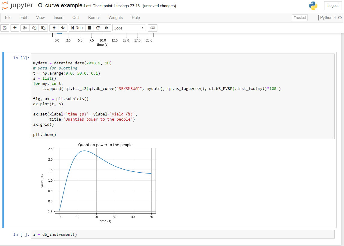
Parametric Yield Curve Fitting

Fit a Nelson-Siegel-Laguerre model and plot instantaneous forward rates:

import ql
import datetime
import numpy as np
import matplotlib.pyplot as plt

mydate = datetime.date(2018, 9, 10)
t = np.arange(0.0, 50.0, 0.1)
s = list()
for myt in t:
    s.append(
        ql.fit_l2(ql.db_curve("SEK3MSWAP", mydate),
                  ql.ns_laguerre(), ql.WS_PVBP)
        .inst_fwd(myt) * 100
    )

fig, ax = plt.subplots()
ax.plot(t, s)
ax.set(xlabel='time (s)', ylabel='yield (%)',
       title='Instantaneous Forward Rates (NS-Laguerre)')
ax.grid()
plt.show()

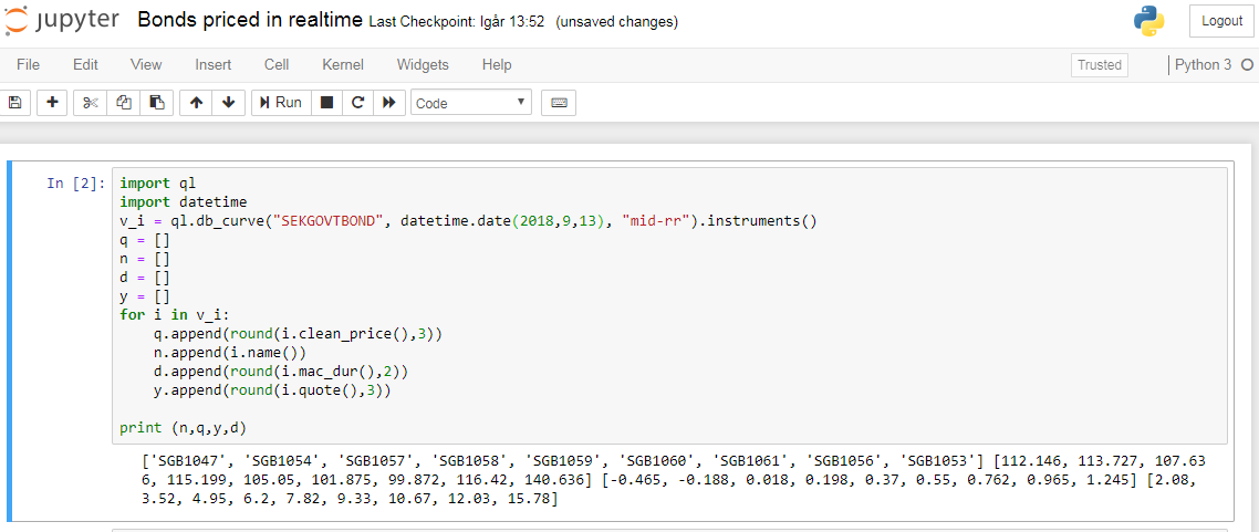
Bond Pricing and Instrument Data

Extract static and pricing data from bonds in a curve:

import ql
import datetime

v_i = ql.db_curve("SEKGOVTBOND",
                   datetime.date(2018, 9, 14),
                   "mid-rr").instruments()

for i in v_i:
    print(f"{i.name():20s}  price={i.clean_price():8.3f}  "
          f"yield={i.quote():6.3f}  dur={i.mac_dur():5.2f}")

Historical Price Quotes

Query the database for historical equity prices:

import ql
import datetime

start = datetime.datetime(2018, 1, 1)
end = datetime.datetime.today()
daterange = [start + datetime.timedelta(days=x)
             for x in range(0, (end - start).days)]

q = []
for d in daterange:
    tmp = ql.db_instrument("SHB A:XSTO:SEK", d).quote()
    if tmp is not None:
        q.append(round(tmp, 2))

print(q)

Heston Model Calibration

Calibrate a Heston stochastic volatility model from market data:

import ql

time2mat = [1, 2, 3]
strikes = [80, 90, 100, 110, 120]
fwds = [100, 101, 102]
# Vols are allowed to be incomplete (None for missing)
vols = [[0.3,  0.25, 0.22, 0.25, 0.28],
        [None, 0.22, 0.2,  0.24, 0.25],
        [None, 0.20, 0.18, None, 0.24]]

# Heston initial guess: [v0, theta, rho, kappa, sigma]
initial_guess = [0.025, 0.04, -0.25, 2, 1]

h = ql.heston_calibration()
h.add_data_for_maturity(time2mat, fwds, strikes, vols)

start = ql.now()
result = h.calibrate(
    ql.calibration_target.OPTION_PRICE,
    ql.calibration_weights.VEGA_WEIGHTS,
    initial_guess)
stop = ql.now()

print(ql.pretty_duration(start, stop))
print([result.v0(), result.theta(), result.rho(),
       result.kappa(), result.sigma()])

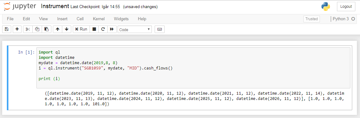
Cash Flow Extraction

Get cash flows from a bond instrument:

import ql
import datetime

mydate = datetime.date(2019, 9, 9)
cf = ql.instrument("SGB1050", mydate, "MID").cash_flows()
print(cf)
# Returns: ([dates...], [amounts...])

Python-QLang Interoperability

A few things to be aware of when using QLang/Quantlab from Python:

• No vector expansion: Vector and matrix function expansion does not work in Python. You must loop in Python.

• Date types: The date type in Python has no overloaded +/- operator with QLang dates, so ql.today() - 1 does not work. Use datetime for date arithmetic.

• Nullable parameters: Variables passed as option(nullable) in QLang can be omitted in Python.

• Out arguments: Variables passed as “out args” in QLang will be returned in a Python tuple.

• Function overloading: Fully supported from QLang to Python (since Quantlab v3.1.2016).

• Class constructors: If a class has no create function, one is dynamically created for Python export.

Using “out arguments”

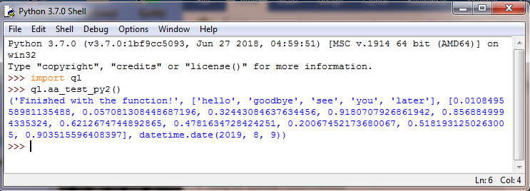
In QLang, “out” arguments return data via the workspace. In Python, they are returned as a tuple. If the function also has a return value, it is the first element:

// QLang function with out args and return value:
out string aa_test_py2(out vector(string) n,
                       out vector(number) r,
                       out date d)
{
    n = ["hello", "goodbye", "see", "you", "later"];
    r = rng_vector(10);
    d = today();
    return "Finished with the function!";
}

Calling from Python:

>>> import ql
>>> ql.aa_test_py2()
('Finished with the function!',
 ['hello', 'goodbye', 'see', 'you', 'later'],
 [0.0108..., 0.569..., ...],
 datetime.date(2019, 8, 9))

Note: All “out arguments” in QLang are by default option(nullable), so in Python the user does not have to declare and pass empty variables.

Function overloading with nullable

What happens if you have overloading of a function with option(nullable) arguments? In the below construction only the first test will be available when calling it using test(None, None) or test() or test(None) as neither of these calls can tell which of the functions you want to address:

void test(out string s, out string t) { s = "test 2"; t = "t"; }
void test(out string s) { s = "test 1"; }

Exporting modules

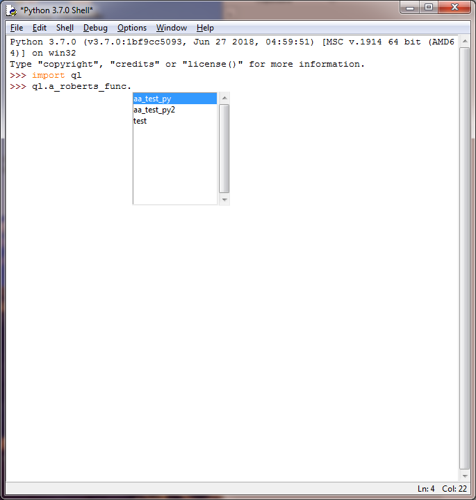
From version 3.1.2021 of Quantlab, library modules are also exported to Python. They appear as namespaces:

>>> import ql
>>> ql.a_roberts_func.aa_test_py(5, 3)
>>> ql.a_roberts_func.test()

Debugging QLang from Python

It is possible to debug a Python session’s QLang code directly in the QLang debugger/editor.

Start a Python-aware Quantlab debug session:

C:\Algorithmica\Quantlab> quantlab-64 -Z

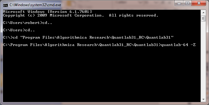
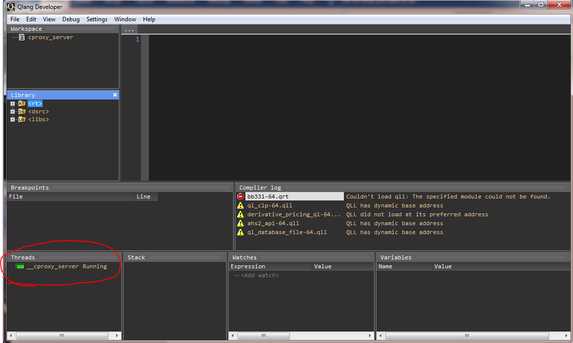
This opens the Quantlab Debugger with a “cproxy_server” process thread started. This process listens for Python processes that initialize Quantlab libraries using import ql.

Multiple Python sessions can be started from different environments (Jupyter Notebook, Python IDLE, VS Code). Set breakpoints and debug in Quantlab as normal.

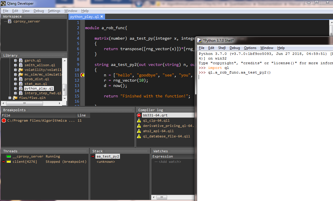
Note: The Quantlab Editor/Debugger will be in “lock-down” mode during the debugging session. It will not allow changes or re-compiles of the QLang code.