Case studies

The following case studies are aimed to illustrate common financial calculation subjects. Most of the examples are programmed using the short form for functions, i.e., one-row functions. Each example corresponds to a workspace file in the folder \Quantlab\examples\workspaces\.

Producing a zero coupon curve: zero_curve.qlw

In this example we will take a set of instruments - a yield curve - and calculate zero coupon rates using the bootstrap method. The zero coupon rates are then plotted against time to maturity in order to produce a zero coupon curve.

Here is a function that solves the problem:

out series<number>(number) zero_curve(curve_name c_n, date trade_d)
{
   disc_func f_r = bootstrap(curve(c_n, trade_d));

   return series(t: 0.1, 10, 0.1; f_r.zero_rate(0, t, RT_EFFECTIVE));
}

In the first line of code of this function, we create a curve using a curve name and a trade date. Then we apply the bootstrap function which gives us a fit_result object z_c which contains all information on the zero coupon rates. What Quantlab does when it performs this row, is that it searches in the database for a curve with the curve name stored in the parameter c_n for the date trade_d. It then collects all static data for the instruments on the curve on the specified trade date and performs a zero coupon calculation using the bootstrap method.

In order to plot a graph, we have to produce a series of zero coupon rates. Here we take a maturity range from 0.1 years to 10 years with a step size of 0.1, and calculate the zero coupon rate for each maturity using the method zero_rate of the fit_result object.

We have chosen to plot the effective zero coupon rate. The zero coupon rate starts at the trade date and matures at t years later. As there is no forward start the first argument of zero_rate is set to 0.

The function can be attached to a graph. Although there are no common parameters, you can rename the parameters by clicking the right mouse button, choosing parameters options and then create two controls; one for the trade date, one for the curve name. For more information about merging parameters, see An example of how to merge parameters to common controls.

Depending on what curves are defined in your database, you can choose a curve and get a zero coupon curve based on that collection of instruments.

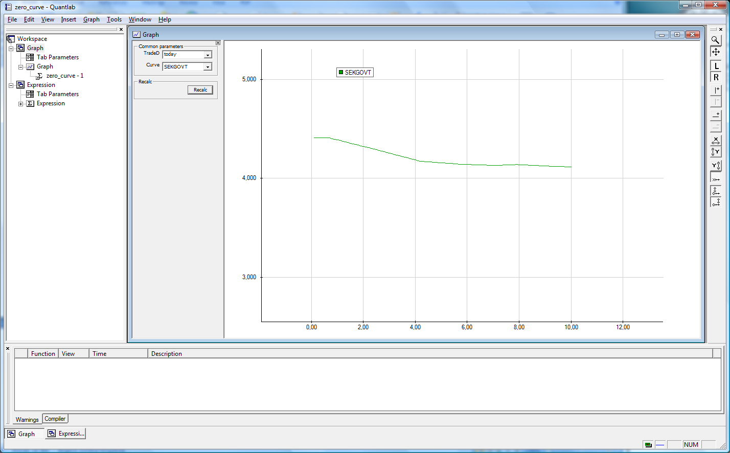
Correctly applying the example should give a workspace with yield curve and date controls.

Zero coupon curve with blending and choice of methods: zero_curve2.qlw

The previous case can easily be extended with the option to choose the zero coupon method. Let’s say you will give the end-user the possibility to choose between the bootstrap, Nelson-Siegel, and Maximum Smoothness methods. Then the zero coupon function in the previous case can be extended like this:

out series<number>(number) zero_curve(curve_name c_n1,
                                      curve_name c_n2,
                                      date trade_d,
                                      string method,
                                      quote_side qs)
{
   curve c = blend_curve(curve(c_n1, trade_d, qs), curve(c_n2, trade_d, qs));

   disc_func f_r;

   if(method=='Bootstrap')
       f_r = bootstrap(c);
   else if(method =='Nelson-Siegel')
       f_r = fit(c, ns(), WS_PVBP, 2);
   else if(method == 'Max Smoothness')
       f_r = max_smooth(c, SMOOTH_C2);
   else
       throw(E_INVALID_ARG, 'Unknown zero coupon method');

   return series(t: 0.1, 10, 0.1; f_r.zero_rate(0, t, RT_EFFECTIVE));
}

We have also taken the opportunity to extend the curve creation with a blending function: This function will take a curve with short maturities and a curve with long maturities and merge them. If there are overlapping instruments, they will be removed from the short curve. For other blending options, see the Function browser. The parameter qs gives the possibility to choose among pre-defined quote sides (bid, ask or mid).

Instead of letting the user manually type the strings for the zero coupon methods we can create a list from which it is possible to make a selection:

out vector(string) methods() = ['Bootstrap', 'Nelson-Siegel', 'Max Smoothness'];

This vector function can then be attached to the string control in the user interface that corresponds to the parameter method.

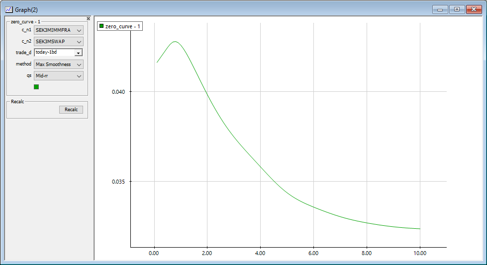
The Maximum smoothness method applied to a blending of two curves.

A zero coupon studio: zero_studio.qlw

This example is a more elaborate version of the preceding zero coupon workspaces. We will not go through the code row by row but give some general comments.

The most important calculation is done in the void function calc_zero which sets the global fit_result variable g_f_r to the result of a zero coupon estimation of the chosen type. Then there are a number of functions that use the global variable to produce the zero coupon curve, the forward curve or zero coupon implied yields for the bonds. As the void function is evaluated first, all other functions will always use the global variable when it is updated with the most recent real time quotes and user input.

However, if a function only presents data that is based on a global variable, it will not be triggered by real time updates, therefore the first row of these functions creates a curve of the relevant instruments. If today’s date is chosen this will make these functions triggered by real time updates in any of the instruments on the curve.

In the user interface, we have merged parameters for all functions in the tab parameter pane. For the zero coupon models and the weighting methods we have used fill-attachments on the merged controls.

Pricing a bond relative to a benchmark curve: bond_pricing.qlw

Often fixed-income instruments are priced relative to a benchmark. Either this can be a single instrument where you simply calculate the yield spread between the two instruments, or a whole curve. In the latter case you have to calculate the corresponding zero coupon benchmark curve and then price all cash-flows of the selected instruments using the zero coupon rates. This gives a fair value of the bond, if it were an instrument on the benchmark curve. The spread between the corresponding zero-curve implied yield and the market yield is therefore an accurate measure of the spread to the benchmark curve.

In this example we will produce a graph of the daily spread between a bond and a benchmark curve during a chosen time period.

As in example Producing a zero coupon curve: zero_curve.qlw, we must first create a curve using a curve name and a trade date. Then we apply the bootstrap function which gives us a fit_result object which contains all information on the zero coupon rates:

disc_func zero_rate_structure(curve_name c_n, date trade_d)
{
    return bootstrap(curve(c_n, trade_d));
}

When this function is calculated, Quantlab searches in the database for a curve with the curve name stored in the parameter c_n for the date trade_d. It then collects all static data for the instruments on the curve on the specified trade date and performs a zero coupon calculation using the bootstrap method.

Now, we want to calculate the spread between the bond and the benchmark. The following line of code solves that problem:

return i.yield() - i.yield(zero_rate_structure(c_n, trade_d));

The function first retrieves the market yield of the bond and then subtracts the yield implied from the zero coupon function. Note that this yield is calculated from the sum of the present values of all cash-flows of the bond, valued using the zero coupon curve.

Finally, we want to plot this spread for each day during a chosen time period:

out series<date>(number) spread_series(curve_name      c_n,
                                       instrument_name i_n,
                                       date            from_d,
                                       date            to_d)
{
   return series(d : from_d, to_d; yield_spread(c_n, instrument(i_n, d), d));
}

Here, we construct a series from the date from_d to the date to_d and call our spread function for each day in the date range.

On each day in the date range the following steps are performed:

• Retrieve the instrument data from the database.

• Retrieve the curve data from the database (what instruments are on the curve on that specific date).

• Retrieve the instrument data for each instrument on the curve.

• Retrieve market prices for all instruments above.

• Calculate a zero coupon curve (a disc_func or fit_result).

• Calculate the present value of all cash-flows of the bond.

• Convert the present value to an equivalent zero-implied yield, using the calculation method of the bond.

• Calculate the spread between the market yield and the zero-implied yield.

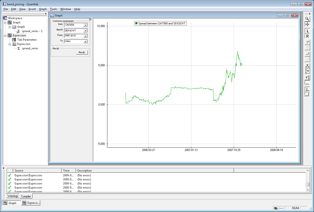
The example - showing a Swedish mortgage bond spread to the SEKGOVT curve.

An instrument table with spreads to a benchmark curve: bench_spreads.qlw

In this example we will make use of an instrument table. This is a special-purpose table where each row corresponds to a particular instrument and each column corresponds to a function that operates on the instruments. Actually, the function takes as input parameter a vector of instruments which corresponds to all rows in the table. See The instrument table for general information about the instrument table.

First, create an instrument table by choosing Insert and then Instrument Table in the menu bar. In the Instrument Table dialog you will be able to decide which yield curve or which instruments that should form the instrument vector for the table. You can also choose trade date and quote side for the instruments. These settings can be changed in the parameter pane if you press the button called Modify.

The first column in an instrument table typically contains the instrument names. This can be done by attaching the following expression to the instrument table:

out vector(instrument_name) names(vector(instrument) i) = i.name();

The input parameter i is set by Quantlab according to your choice in the Instrument Table dialog. In the same manner you can create functions that will give the maturity dates and the yields of the instruments:

out vector(date) mats(vector (instrument) i) = i.maturity();

out vector(number) yields(vector (instrument) i) = i.yield();

For the calculation of spreads, we will proceed similar to the example in Zero coupon curve with blending and choice of methods: zero_curve2.qlw:

out vector(number) yield_spread(curve_name         c_n,
                                date               trade_d,
                                vector(instrument) i)
{
   disc_func f_r = bootstrap(curve(c_n, trade_d));

   return i.yield() - i.yield(f_r);
}

Note that in the yield spread function we have changed the instrument parameter to a vector of instruments. The vector of instruments has to be the last parameter of the function. In order to only do the bootstrap calculation once, we save the fit_result object in the local variable f_r.

If you attach all these functions to the instrument table you will get a table of spreads to a given benchmark curve.

Probably, you want to see the yields in percentage points and the spreads in basis points. This can be done by right-clicking the appropriate column header and choosing Number format. In the Number format dialog you can choose to multiply all numbers in the column by a factor, for example 100 or 10,000.

You can also right-click to reach menus for formatting the cells in the table and the column header text. For example, in the Column display dialog you can set the display name of the spread column to “Spr to ” and then double click on the c_n parameter in the list box to the right in order to get the current curve name in the header. The column header will then be “Spr to SWAP” if you have chosen a curve called SWAP.

Extending spread calculations with user input: bench_spreads2.qlw

The previous example can easily be extended with a possibility to manually input the yields. In order to get relevant yields to start with the workspace will present the market yields in the input column. To be able to differentiate between the two cases (1) the first time the calculation is done, or (2) when a manual input is done, we have introduced a global variable g_initiated:

logical g_initiated = false;

out vector(number) yield_spread(curve_name         c_n,
                                date               trade_d,
                                out vector(number) yields,
                                vector(instrument) i)
{
   if(!g_initiated)
   {
       yields = i.yield() * 100;

       g_initiated = true;
   }
   disc_func f_r = bootstrap(curve(c_n, trade_d));

   return yields/100 - i.yield(f_r);
}

When the workspace is opened and the function is evaluated for the first time, g_initiated is false, but each time the user makes an input in the yields column, g_initiated will be true. Thus, the workspace will use the market rates for the first time and then the user input.

As the function is attached to an instrument table, the input vector yield_spread will automatically have the same length as the instrument vector i.

Calculating covariances: covariance_matrix.qlw

This simple example shows how to use vector expansion and how you can use vector input in tables. We will calculate a covariance matrix and a correlation matrix using price quotes for some instruments.

We start by creating a time series with logarithmic changes of quotations on one instrument:

out series<date>(number) log_series(instrument_name i_n, date from_d, date to_d) =
     change(series(t : from_d, to_d; log(instrument(i_n, t).quote())));

The function change operates on the series and takes the difference between each value and the previous one. If one of the values is Null, then the value of the change also is Null.

This function can be called using vector expansion in order to calculate the covariance matrix:

out matrix(number) covar_matrix(vector(instrument_name) i_n, date from_d, date to_d) =
    covariance(log_series(i_n, from_d, to_d));

This function can be attached to a table where you will have to set the number of rows in the input vector of instrument names. This is cone by right-clicking on the corresponding column header and selecting Input parameters.

If we instead want to have the correlation matrix we write:

out matrix(number) corr_matrix(vector(instrument_name) i_n, date from_d, date to_d) =
    correlation(log_series(i_n, from_d, to_d));

Creating a simple portfolio Value-at-Risk function: Portfolio_VaR.qlw

This example will use the matrix calculation possibilities in order to calculate a Value-at-Risk measure for a small portfolio. Actually we will test three different VaR models.

In order to get easy access simulation possibilities, we will expose the most important parameters to graphic interface. The function definition nmb looks like this

out vector(number) myRisk(vector(instrument_name) i_n,
                          vector(number)          w,
                          number                  conf,
                          number                  horizon,
                          date                    startdate,
                          date                    enddate)

The parameters are instrument names and their weights and a confidence level and horizon number of days. The dates startdate and enddate are used to choose the date-range for the covariance matrix calculation.

We will use the fact that a series expression can take a vector of instruments as input and return a series of vectors of numbers. The objective is to extract the time series (the clean price) for the chosen instruments and the period specified between startdate and enddate. We also take the logarithmic changes:

series<date>(vector(number)) price_series =
   series(d:startdate,enddate;instrument(i_n,d).clean_price());

series<date>(vector(number)) log_series = change(log(price_series));

We can now create the covariance matrix from the logarithmic changes. To analyse the difference between VaR methods using different time weighting, we create two covariance sets. The first row produces a standard set and the second a RiskMetrics set.

matrix(number) Cov = covariance(log_series);

matrix(number) CovExp = covariance_exp(log_series,0.94);

As a third method, we compute the daily portfolio returns as a percentage. Multiplying the time series of vectors with the weights will return the daily portfolio value. For each day there will be an inner product of the returns and weights:

series(number) dPortf = change(log(price_series * w));

We are now ready to conclude and return the three equivalent Value-at-Risk figures together with the sum of weights:

number A = sqrt(w * Cov * w * horizon) * inv_normal(conf);

number B = sqrt(w * CovExp * w * horizon) * inv_normal(conf);

number C = std_dev(dPortf) * sqrt(horizon) * inv_normal(conf);

number D = v_sum(w);

// return a vector with the results

return [A, B, C, D];

We will not give a lesson on Value-at-Risk formulas here but concludes that we again use Quantlab’s series and vector capabilities to write the formulae in short-form.

Calculating tail rates: tail.qlw

This is another example that illustrates some vector functions. We will calculate tail yields for some chosen yield curves. A tail yield is a zero-coupon forward rate between the maturity dates of two consecutive bonds. In order to perform the calculations we have to have two vectors with the settlement dates and the maturity dates for the forward rates, respectively.

First we define two simple help functions:

disc_func boot(curve_name c, date d) = bootstrap(curve(c, d));

vector(date) mat(curve_name c, date d) = curve(c, d).instruments().maturity();

With the second function we can take out the settlement dates and the maturity dates for the forward rates. The question is now how to extract the correct settlement and maturity dates for the tail rates. The first settlement date is the maturity date of the first bond and the last settlement date is the next-to-last maturity date. For the maturity dates of the tail rates it’s the opposite: The first is the next-to-first maturity date among the bonds and the last is the last maturity date of the bonds. This can be solved by using the sub_vector function:

vector(date) settle(curve_name c, date d) = sub_vector(mat(c, d), 0, v_size(mat(c, d)) - 1);

vector(date) matur(curve_name c, date d) = sub_vector(mat(c, d), 1, v_size(mat(c, d)) - 1);

Remember that vectors are indexed starting at 0. In order to calculate the tail rates we use bootstrap and extract the relevant zero coupon yields:

vector(number) tail(curve_name c, date d) = boot(c,d).zero_rate(d,
                                                                settle(c, d),
                                                                matur(c, d),
                                                                RT_SIMPLE, DC_ACT_360) * 100;

In order to plot the tail yields versus the maturity dates we use the following function:

out vector(point_date) tail_graph(curve_name c, date d) = point(matur(c, d), tail(c, d));

To get labels with instrument names the function matur is attached to the tail_graph functions in the graph.

If we want to look at a particular tail rate development over time we can write:

out series<date>(number) tail_series(curve_name c,
                                     instrument_name i1,
                                     instrument_name i2,
                                     date from,
                                     date to)
                                     =
   series(d: from, to; boot(c,d).zero_rate(d,
                                           instrument(i1, d).maturity(),
                                           instrument(i2, d).maturity(),
                                           RT_SIMPLE,
                                           DC_ACT_360) * 100);

Obviously, the maturities of two bonds are required to calculate one tail rate.

Has the market been wrong or right?: expectations.qlw

This is an example of how you can create quite interesting graphs with a very limited amount of work. We are going to plot a graph of the development of the 90 days rate, together with some graphs showing the market’s expectations of the same rate, i.e., forward rates.

First we define our zero coupon function, for example the following:

fit_result my_fit(curve c)
{
   fit_result f_r;

   try
       return fit(c, ns_svensson(), str_to_std_weights('pvbp'), 2);
   catch
       return f_r;
}

By using the norm equal to 2 in the fitting algorithm, price discrepancies are measured using the sum of squares.

This function will be used in two other functions. The first one deal with the historical time series of the fixed short rate:

out series <date>(number) z_series(curve_name cn,
                                   date       from,
                                   date       to,
                                   number     tenor)
{
   return series(t:from, to; my_fit(curve(cn, t)).zero_rate(t,
                                                            t,
                                                            t + tenor,
                                                            RT_SIMPLE, DC_ACT_365));
}

When dropped in a graph window this function will plot the simple Act/360 rate with a maturity time given by tenor, in days, for the time period from the from date to the to date.

Then we want to add the market expectations at some given dates. This can be done by plotting the forward curves, starting at different dates. We write a function for forward curves:

out series<date>(number) z_c(curve_name cn, date d, number tenor)
{
   curve c = curve(cn, d);

   fit_result f_r = my_fit(c);

   return series(t:d, d + 360; f_r.zero_rate(d, t, t + tenor, RT_SIMPLE, DC_ACT_365));
}

Given a date d and a tenor, this function plots a curve with one year’s length (the range is 365 days), showing at date d the rate from time t to time t plus the tenor.

Drag several instances of this function to the same graph window as the function above. Then click the right mouse-button and choose Parameters options. Merge the appropriate parameters (for example the curve name and the tenor), see An example of how to merge parameters to common controls. If you then choose dates for the forwardcurves during the period for the first function you will get a graph looking like this:

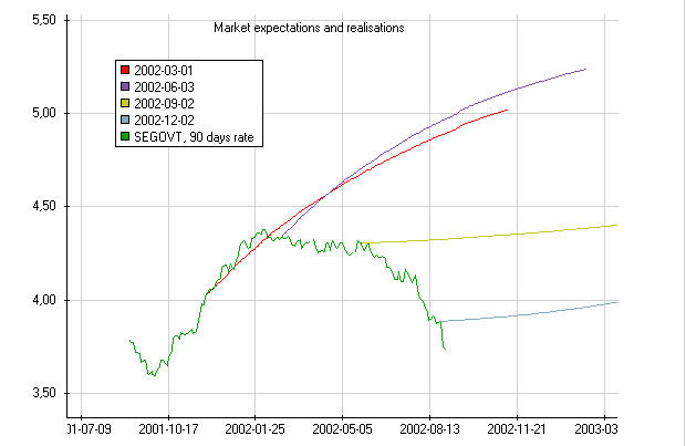
In this case the market was right about the rising rates during the end of 2001 but then it has continuously over-estimated the future short rates.

If the forward curves look rough it may be because of omitted weekends in the time scale. Click the right mouse button on the graph background and choose Graph Properties and the tab Holiday. Unclick the option Hide holidays.

As we have defined one single function that does all zero coupon calculations we can change this to bootstrap or any other type of model and all calculations will remain consistent in the workspace.

Another change you might want to do is to let the user choose between rate types and day count conventions, which is done by introducing parameters for those choices.

Creating an intra-day chart: intraday_graph.qlw

This is an extensive example using global variables for the storage of intraday data. The purpose of the workspace is to draw a graph of the quoted price of an instrument using each intra-day tick.

The kernel of the workspace consists of the following global variables and function:

// This variable is used to see when the user changes instrument
instrument_name i_name;

// This global variable stores the vector of quotes
vector(point_timestamp) v;

// Shows an instrument's quotes in a graph in real time
out vector(point_timestamp) quote_vector(instrument_name i)
{
   number n;
   number quote = instrument (i, today()).quote();

   // If the vector is empty we must create it
   if (null(v) || i_name != i)
   {
       vector(point_timestamp) tmp[1];

       v = tmp;
       n = 0;

       i_name = i;
   }
   else
   {
       n = v_size(v);
   }

   /* If the vector has less than two points
    we add the new point */

   if (n < 2)
   {
       if (n == 0 || v[0].y() == quote)
       {
           push_back(v, point (now(), quote));
       }
       else
       {
           // n == 1 && v[0].y != quote
           resize(v, 3);

           v[1] = point (now(), v[0].y());
           v[2] = point (now(), quote);
       }
   }
   // Otherwise points are added only to
   // reflect any changes
   else
   {
       if (v[n - 1].y() == quote)
       {
           if (v[n - 1].y() == v[n - 2].y())
           {
               v[n - 1] = point(now(), quote);
           }
           else
           {
               push_back(v, point (now(), quote));
           }
       }
       else
       {
           resize(v, n + 2);

           v[n] = point(now(), v[n - 1].y());
           v[n + 1] = point (now(), quote);
       }
   }
   return v;
}

If attached to a graph this function will extend the tick-graph each time there comes a real-time update. If an update has the same value as the preceding one, the x-value will be changed to the new time-stamp without adding a new point. The result will be a typical graph consisting of horizontal and vertical lines.

The global vector v holds the graph data in the form of the Qlang type point_timestamp. It is updated each time the function is called, either by the real-time input or by the user.

The global instrument name i_name is used to check whether the user has changed the instrument which should trigger a complete reset of the graph.

The workspace also draws horizontal lines for closing price and updated maximum and minimum.

Note

Attaching multiple instances of the function created above to a graph will not work properly since they will both share the same instance of the global variable.

Using function pointers and classes: fp_test.qlw

In this example we give some ideas of how to use a couple of new features in Quantlab 3.0: Function pointers and object classes.

We begin by implementing a generic delta function which calculates a numeric delta by calling the pv-function of an imagined class:

number calc_delta(object<1> pos, number function(object<1>, number epsilon) pv)
{
   number epsilon = 0.0001;

   return (pv(pos, epsilon) - pv(pos, 0))/epsilon;
}

This function assumes that there exist a member function pv that returns the present value, given a small disturbance epsilon. The syntax object<1> pos means that this argument is a class object of any type - which in this case must implement the pv-function in a meaningful way.

Let’s try this out by implementing a simplified derivative class and it’s present value function. Note that we can now implement a delta member function by calling the generic delta function above and refer to our member function for the present value by the use of a function pointer. We begin with the derivative class:

class derivative
{
   // Member functions
   number pv(number epsilon);
   number delta();

   // Members
   number price;
};

derivative derivative(number price)
{
   derivative d = new derivative;
   d.price = price;

   return d;
}

number derivative.pv(number epsilon)
{
   return log(price+epsilon); // A very strange pv indeed
}

number derivative.delta()
{
    return calc_delta(this, &derivative.pv);
}

Please note that last line where we use this to refer to the class object and supplies the calc_delta function with a reference to our present value function.

We can now create a derivative object and return the delta value:

out number test_derivative(number price)
{
   derivative d = derivative(price);

   return d.delta();
}

A condensed market page: market_page.qlw

This is an example of how to build a market page with unlimited number of tables showing quotes for financial instruments with several price contributors. It uses the test_rgb object to highlight quote changes.

The function instr(curve_name c_n, date d) can be used repeatedly for creating new instrument tables, given different curve names. Typically d is today(). The function stores the RICs of the instruments in a global list (a map object). Each time there is a new instrument it is added to the list. So, all instrument tables share the same list of RICs.

In the function format_yield(string ric) a string_rgb object is produced with formatting depending on the recent history of changes in the quote. This function is called by the out-function yield(string contributor, vector(instrument) i) which appends a contributor to the RIC.

When formatting the instrument tables it is convenient to transpose the table, to hide the parameter list and to use minimal frames. Then you can get something like the tab below:

An example of a market page showing Swedish bonds.

The header of the table (which actually is the attachment name(vector(instrument) i)) consists of the last two characters in the instrument name and the quote difference from yesterday’s closing. This special header may of course have to be changed for other markets in order to be meaningful. Also the database name (in our case QLDemo) which gives the RICs has to be changed to your database name (i.e., ODBC source).