Programming in Quantlab using Qlang

The Quantlab language Qlang makes financial programming easy! Qlang is designed to work with time series data vectors and matrices. Included in Qlang is also an extensive function library with many tailor-made fixed income functions that makes programming fast and efficient.

Programming in Quantlab follows these basic steps:

1. Write code in an expression editor

2. Check and compile the code [by pressing F7, or choosing Exp, Compile]

3. If code compiled correctly, the “out functions” appear in the Workspace browser

4. Drag and drop the functions from the Workspace browser to graphs and tables

When programming is finished and workspaces have been created, they are ready to be distributed to others. Everyone using Quantlab, either Developer or User Edition, can now run all analytics of the workspace presented in graphs and tables.

A simple example

Let’s look at a simple function that adds two numbers:

number my_add(number x, number y) = x + y;

In order to make this function available for presentation in tables or graphs the keyword out is used, written at the start of the function definition:

out number my_add(number x, number y) = x + y;

If you write this function in an expression window (Insert - Expression) you will be able to compile the code by pressing F7. As the code is correct you will not get any warnings. Try to change the code to something incorrect, for example:

out number my_add(number x, number y) = x + y +

If you then press F7 again, you will get an error message (if messages have not been switched off in under options | messages).

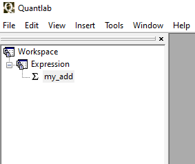
Change back to the original version of the function, recompile the code and look for the Workspace window. In the Workspace window (View - Workspace) you will find a + sign. If you click the plus sign, you will find the function my_add. This function is available to attach to a table. To do so, insert a new table (Insert - Table) and give it a name. Then drag the function my_add (using the left key of the mouse) to the table window and drop it there. Two Number Edit Boxes will appear next to the table, one for each parameter of the function, and these are used for choosing the values of x and y. Enter two numbers in the boxes and press Recalc to make Quantlab evaluate your function and show the result in the table.

Chapter Output - tables and graphics explains more about how to format tables and graphs.

Keyword list

This section is a summary of the keywords that form the language base. Keywords are marked with blue when written in the expression editor. (In default appearance mode. See Settings | Appearance for more options.) Note that a description on each keyword can be found in the function browser.

The keywords Module, Public and Import are used for the management of expressions.

module	The module keyword creates a namespace of functions.
public	The public keyword assigns a function to be available outside a module.
import	The import keyword loads the public functions of a module so that they become local functions.

The keyword Return is used when defining functions in the standard form.

return

The return keyword terminates the current function call and returns the value or object following it. See Standard function definition.

The keyword void is for defining procedures.

void	The void keyword replaces the return value type for a function that does not return any value. See Standard function definition.

The keyword out is special for Qlang and used for making functions available in the user interface.

out	The out keyword assigns a function to become available for attachments to graphs or tables after compilation. See Function parameters for the use on parameters.

The keyword option is special for Qlang and used for certain options for variables and functions.

option

option(nullable) is used in a function definition before a parameter name to make the function possible to call with a null value in that parameter. option. option (category: <string>) is used immediately after the function header in a library file to indicate what category the function shall appear in within the Function browser. The string contains the name of the category, either an existing category or a new one. option (com_name: <string>) is used immediately after the function header in a library file to publish the function to the COM interface (for use in excel or C#) using a user defined name. This is necessary if functions in library are overloaded as COM does not allow for overloaded functions.

The keywords if, switch, else, do, while, for, break and continue are used for flow control.

if else	The if and else keywords are used for conditional expression evaluation. See If, else, do and while.
switch	The switch keyword is used when there are several cases in a comparison situation. See The switch statement
while	The while keyword is used for conditional loops with initial condition test. See If, else, do and while.
do while	The do while keywords are used for conditional loops with final condition test. See If, else, do and while.
for	The for keyword is used for unconditional loops. See The for loop.
break	The break keyword terminates the smallest enclosing loop statement (do, for, or while) in which it appears.
continue	The continue keyword terminates the current iteration of the smallest enclosing loop statement (do, for, or while) in which it appears, and the execution continues with the next iteration.

The keywords Try and Catch are used for error handling.

try	The try keyword introduces a code section in which errors are expected to occur. See Error handling: Try and catch.
catch	The catch keyword introduces a code section that takes care of the errors in the preceding try section. See Error handling: Try and catch.

The keywords String, Matrix and Vector are used for creating specific types.

string	The string keyword assigns a variable, function or a function parameter to be a string. See Basic types.
matrix	The matrix keyword assigns a variable, function or a function parameter to be a matrix. See Vectors and matrices.
vector	The vector keyword assigns a variable, function or a function parameter to be a vector. See Vectors and matrices.

These keywords are always used in connection with an object type. For example, to create variable which is a vector of numbers, you write

vector(number) my_variable;

The keyword Series is a special Qlang feature used in particular for time-series calculations.

series

The series keyword creates a series of elements by evaluating an expression over a range. The dimension of the series is equal to the number of ranges. See Series.

The keywords Object and New are used when defining objects.

class	The class keyword is used when defining an object class. See Creating new classes.
object	The object keyword is used when defining an object class. See Creating new classes.
new	The new keyword is used when creating an instance of an object. See Creating new classes.

The keywords typedef and enum are used for defining types.

typedef	The typedef keyword is used when giving new names to types. See Definition of types.
enum	The enum keyword is used when creating enum lists. See Declaring your own enum types.

The keyword Function is used for function reference in function definitions.

function

The function keyword refers to a function parameter in a function definition. See Standard function definition.

The keyword operator is used when defining operators, typically for objects.

operator

The operator keyword is used when defining operators, see Example of classes and operators.

Functions

Functions can be defined in two ways, in the standard way and the compact way. In the standard function definition, the syntax resembles very much the syntax of C++ or similar languages, in the compact form the function definition is written by using only one expression. Both forms can be used in the same expression window.

Standard function definition

The standard way of defining a function looks like this:

return_value_type function_name (parameter_type1 parameter_name1, ...)
{
   < function body >

   return < expression >;
}

The function is defined by declaring the return value type, the function name followed by a parenthesis, and then a function body. Inside the parenthesis all the function parameters are defined by writing their types and names. Note that each parameter requires its own type definition, and that these types are specific for Qlang. Within the function body the usual variable declarations and operating statements are written, each ending with a semi-colon. The function returns the value of the expression that follows immediately after the keyword return.

For example, a function adding two numbers:

out number my_add(number x, number y)
{
   return x+y;
}

The return value type must be declared as any of the Qlang types. If the return value type is set to void and the return statement is omitted, the function returns no value:

void function_name (parameter_type1 parameter_name1, ...)
{
   < function body >
}

The keyword out is used to make a function available for attaching to graphs or tables. For example, the following function could be attached to a table in order to display a multiplication table:

out vector(number) mult(number x)
{
     vector(number) y = [1, 2, 3, 4];

     return x * y;
}

Compact function definition

This is an alternative way of defining functions, which is useful for simple expressions. It is written starting with a return value type and a function name, followed by a parenthesis containing the parameters, and then an equality sign. After the equality sign must be a complete function expression. The function takes the following form:

return_value_type function_name (parameter_type1 parameter_name1, ...) = <function_expression>;

Note that the expression ends with a semi-colon. The my_add example used earlier would look like this:

out number my_add(number x, number y) = x + y;

These functions are often written in one row, but for the sake of readiness, they can be written in several rows:

out number my_add(number my_x_parameter, number my_y_parameter) =
my_x_parameter + my_y_parameter;

New in version 3.1.2048: The generic return type “auto” can be used. It is used in the same way as in C++.

out auto mult(number x)
{
   vector(number) y = [1, 2, 3, 4];

   return x * y;
}

Instances of functions

When a function is attached to a table or a graph an instance of the function is created. You may have several instances of the same function in the same graph or table. In the calculations and user interface, Quantlab will treat them as separate functions that may or may not use the same input parameters. Only when the code, i.e. the definition of the function, is changed this will affect all function instances.

Function parameters

Function parameters are defined by the type followed by the parameter name, as described in Standard function definition. There is also a possibility to define optional parameters with a default value by setting these parameters equal to an expression, for instance:

number my_add(number x, number y = 1)
{
   return x+y;
}

out number test_my_add(number x)
{
   return my_add(x);
}

The first function, my_add, has one optional parameter y which is defaulted to 1 if not set, as in the second function test_my_add. The default value may also be something more complex, for example a function call:

number default(number x)
{
   return x*2;
}

number my_add(number x, number y = default(2))
{
    return x+y;
}

out number test_my_add(number x)
{
   return my_add(x);
}

In this example we have defined a separate function called default which calculates the default value for the function.

When attaching functions to graphs or tables, all parameters, including optional ones are displayed, without default values.

When calling functions, the function parameters are by default copies (for number, date and logical) or copies of references (for string and object) of the original variable.

In the following example, the function f2 returns 0 as function f1 only changes a copy of the original variable.

void f1(number c)
{
    c = 1;
}

out number f2()
{
   number b = 0;

   f1(b);

   return b;
}

Using the keyword out before a parameter definition will cause that parameter to be referring to the original variable (for number, date and logical) or original reference (for string and object), allowing change of the external environment. This is similar to the Pascal VAR parameter and the C++ way of declaring a parameter as a reference (using &).

In the following example, the function f2 returns 1 as function f1 changes the value of the original variable.

void f1(out number c)
{
   c = 1;
}

out number f2()
{
   number b = 0;

   f1(b);

   return b;
}

Calling functions

There are a large number of pre-defined functions in Qlang for general and financial purposes. These are divided into groups according to their purpose and can be found in the Quantlab function browser. The function browser is made visible from the Quantlab menu bar (View - Function Browser).

Both user-defined functions and pre-defined functions are called similarly to common programming languages. For example the user-defined function my_add in A simple example could be called like this:

result = my_add(2, 3);

if we have defined a variable called result, of the type number.

Important

From version 3.0 and onwards, functions without any parameters must be called using an empty parentheses, for example my_func(). This is a common case for many object member functions.

Function pointers

In Quantlab 3.0 the concept of function pointers is introduced. It is useful in various cases, for example when performing optimisation calculations. Here is an example which uses the minimisation function zero_bisect. See also Creating new classes for information on object classes.

class param_object
{
   // This object contains all parameters that are used for
   // calculating the function f,except for the variable x.

   public:
       number a_param;
};

number f(param_object p, number x)
{
   // The object function
   return -p.a_param*x + 1;
}

out number test()
{
   // Find x that makes f = 0.

   param_object p = new param_object;

   p.a_param = 4;

   number x1 = -3;
   number x2 = 4;
   number tol = 0.001;

   return zero_bisect(p, &f, x1, x2, tol);
}

On the last line we call zero_bisect with a reference to the function f using the &-sign. The function zero_bisect requires that the function that is referenced to (in our case, f) has two parameters: An object and an x-parameter. In this way you can construct a function f that is arbitrarily complicated as long as it is a function of a single variable x.

The following example shows how to define your own function pointers. The function calc below performs any calculation using a function f that takes two parameters. We have defined two such functions: plus and minus. The last function below uses these functions depending on the user input.

number plus (number a, number b) = a + b;
number minus (number a, number b) = a - b;

number calc(number a, number b, number function (number a, number b) f)
{
   return f(a, b);
}

out number test(number a, number b, string method)
{

   if(method == 'plus')
       return calc(a, b, &plus);

   if(method == 'minus')
       return calc(a, b, &minus);
}

The syntax for the declaration of the function pointer is thus:

<return_type> function (<type>param_1, <type> param_2...) function_param_name

More examples of function pointers are found in the case study in Using function pointers and classes: fp_test.qlw.

Local and global variables

In a function, local variables may be declared as in other common programming languages, with or without initialisation, for example:

<function declaration>
{
     number x;

     number y = 5;

     vector(instrument) i;

     ...
}

For global variables the treatment is somewhat more special. Global variables are only common to all calls from functions within the same expression window. An example:

number x;

out number my_function(number y)
{
   if (null(x))
   {
       x = 0;
   }
   else
   {
      x = x + 1;
   }

   return x*y;
}

Each time my_function is called, the variable x will be updated. An extensive example of how to use global variables is discussed in Calculating tail rates: tail.qlw.

Important

It is important to note that multiple instances of functions attached to the same or different tables or graphs will all refer to the same instance of the global variable.

Operators

Common mathematical and logical operators are available in Qlang. Operators work like ordinary functions, for example allowing vector and matrix expansion, see Vectors and matrices.

Arithmetic operators:

+ addition

- subtraction

* multiplication

/ division

^ power (can also be written using the function pow)

Note

The type of multiplication is determined by the operands. A multiplication of two vectors will result in a scalar (so called scalar product). A multiplication of matrices or a matrix and a vector is treated as a matrix multiplication. See Vectors and matrices.

Logical operators:

! logical negation

!= not equal to

&& logical AND

|| logical OR

<,> logical relation operators

== logical equality operator

There is also a simple conditional operator available using the following syntax:

<conditional expression> ? <expression1> : <expression2>

If the conditional expression is evaluated as true then expression1 will be returned, otherwise expression2. For example, the following function will return x if it is positive, otherwise 0.

number my_function(number x) = x > 0 ? x : 0;

Quantlab will perform a short-circuit evaluation of logical and conditional expressions, only executing those that are necessary.

Note

As in many languages, assignment operators are allowed together with the assignment sign (“=”). Such that <variable> /= 10; means divide value in variable with 10.

Also:

+= for add

-= for subtract

*= for multiplication

Data types

Qlang carries a rich family of types, much like any modern programming language.

Basic types

The number of basic types in Qlang is limited for ease of use. Qlang has the following seven basic types.

Type	Description	Literals
number	The basic float numeric type	Numbers are simply entered as they are. Very small or large numbers can be written with mantissa, then d, D, e or E, then the exponent. 1.2e-4 is interpreted as 0.00012, or 1.2 basis points.
integer	Integer type	Same as in other languages. Any indexation for vectors, loops etc starts with 0.
date	The basic date type	Dates are written using # then ISO standard dates. #2000-12-29 is interpreted as the 29th of December 2000.
timestamp	Basic long date including time	Timestamps are written using # with iso date and time down to optional thousands of a second. ex. timestamp tss = #2021-01-01 12:30:22.222;
logical	The basic Boolean type	True or false.
string	The basic character string type	Strings are encapsulated by simple or double quotation marks. Both ‘text’ and “text” are interpreted as strings containing the word text.
month	A month basic type	It is a date without any day reference. e.g. #2023-03.
object	The basic object reference type	No literal.

Of the above basic types, only the object basic type cannot be used directly in variable or function parameter declaration. Instead of the object basic type, the object types described below are used.

This is an example of using some basic types to get different user controls when attached to a table.

out number myFunc(string myStr, number myNum, date myDate)
{
   ...
}

Quantlab recognizes the types and automatically creates appropriate controls.

Object types and member functions

There are many object types available in Qlang. Many of them are financial, such as instrument and curve, but there are a others used for presentation of data, for mathematical purposes and so on.

Objects are generally created as a result of Qlang function calls. They can then be stored in variables or used directly for further function calls. Objects also have member functions, which can be called using a standard dot notation.

Below is an example of a function that returns the yield of an instrument on a specified trade date. An instrument object is created from the information in the database, and then the member function yield() is called to extract the sought yield.

number my_yield(instrument_name i, date tradeD)
{
   return instrument(i, tradeD).yield();
}

Some objects methods have a corresponding function in another object. As an example, both rows below will return the dirty price of an instrument priced from a zero coupon curve model fit of the market rates.

fit_result.dirty_price (instrument);
instrument.dirty_price (fit_result);

Creating new classes

An introduction to working with user-defined classes In Quantlab 3.0 it is possible to create new classes with member variables and member functions. The syntax is very much in line with C++. Below is an example of a definition of an object class that stores two numbers, called my_pair. The object class has a member function that adds the two numbers and a creator with the same name as the object class. The last function can be attached to a table in order to test the object class.

class my_pair
{
public:
   number add();

   number x;
   number y;
};

// Note that you need to declare all member functions inside the class
// definition - as is done with the function add() above.

my_pair my_pair(number x, number y)
{
   my_pair t_n = new my_pair;

   t_n.x = x;
   t_n.y = y;

   return t_n;
}

number my_pair.add()
{
    return x + y;
}

out number test_my_pair(number x, number y)
{
   my_pair p = my_pair(x, y);

   return p.add();
}

The class definition syntax A user-defined class is defined using the following syntax:

class <class name> [ : <class to inherit from> ]
{
   [public:]|[private:]
   ...
   [<name of constructor (i.e. class name)>(<params>);]
   ...
   [virtual <return type> <name of virtual member function>(<params>);]
   ...
   [<name of member function>(<params>);]
   ...
   [<type of member variable> <name of member variable>;]
   ...
};

<class name>.<name of constructor>(<params>)
[: <name of member variable>(<params>),...]
{
   <body>
}
...
<return type> <class name>.<name of member function>(<params>)
{
   <body>
}
...

A class may inherit from another class - called a super-class - by using the familiar : <class to inherit from> notation above.

In a class - as opposed to an object - all members and member functions (including constructors) are declared private: by default. This means that they cannot be accessed by any code outside the class. In order to make them accessible from the outside they need to be within the scope of a preceding public: declaration:

class myClass
{
   public:
       number get_secret_number();
   private:
       number secret_number;
};

Now, the secret_number above can only by accessed through the get_secret_number().

A special type of member function called a constructor is used to initialize the member variables of a class. It is possible to do this using the familiar [: <name of member variable to initialize>(<params>)] notation, as in the following example:

class myClass
{
   public:
       myClass(number n);

       number get_secret_number();
   private:
       number secret_number;
};

myClass.myClass(number n)
: secret_number(n)
{}

number myClass.get_secret_number()
{
   return secret_number;
}

Note that a constructor cannot have an explicit return type, since it implicitly returns the newly created class object.

The virtual keyword declares a virtual member function that can be overridden by any inheriting class as seen in the following example. Note that all virtual member functions need to be defined in all classes - also in the super-class:

class A
{
   public:
       virtual string f();

       string g();
};

string A.f() {return "A.f";}

string A.g() {return "A.g";}

class B: public A
{
   public:
       virtual string f();

       string g();
};

string B.f() {return "B.f";}
string B.g() {return "B.g";}

class C: public A
{
   public:
       virtual string f();

       string g();
};

string C.f() {return "C.f";}

string C.g() {return "C.g";}

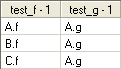
out vector(string) test_f()
{
   vector(A) v = [new A, new B, new C];

   return v.f();
}

out vector(string) test_g()
{
   vector(A) v = [new A, new B, new C];

   return v.g();
}

The output table below shows the difference between the virtual member function f() and the normal member function g():

Scope of class members and the use of this The familiar dot notation is used to access member variables and calling member functions in a class:

A a = new A;

a.my_number = 42; // Accessing one of A:s members

a.f(); // Calling one of A:s member functions

By explicitly naming the class name after the dot it is possible to access member functions or variables that are normally hidden by definitions in inheriting classes. This can be done even if the function is not declared as virtual:

B b = new B;

b.f(); // Calling the f() member function defined in B

b.A.f(); // Calling the f() member function defined in A

It is possible for a member function of a class to obtain a handle to itself by using the this keyword. This can for example used as a parameter in function calls as in the following example:

string func(A a)
{
    return a.f();
}

logical A.func()
{
    string s1 = this.f();

    string s2 = func(this);

    return s1 == s2; // always returns true
}

Please note though, that a member function can always access all of its own member variables directly without using this.

Casting classes When working with class hierarchies it is often useful to convert a handle to a super class object into a handle of the actual base class it belongs to (or any other class in between). This is called a dynamic cast and is performed by using the dynamic_cast operator:

A a = new B; // This is possible since class B inherits from class A

B b = dynamic_cast<B>(a); // Convert into a handle to a B

If the cast is not possible due to the classes not being members of the same class hierarchy it will fail and an error will be thrown.

When writing library files, it is also possible to add new member functions to built-in object classes, see Adding member functions to object classes. More examples of creating object classes are found in the case study in Using function pointers and classes: fp_test.qlw.

Example of classes and operators

Here is a simple example where complex numbers and the + operator is defined in a library file:

class complex
{
   private:
       number r, i;
   public:
       complex(number r, number i);

       number re();
       number im();
};

complex.complex(number r, number i) : r(r), i(i) {;}

number complex.re()
{
    return r;
}

number complex.im()
{
    return i;
}

// Operator overloaded using a member function
complex operator + (complex c, complex d)
{
    return new complex(c.re() + d.re(), c.im() + d.im());
}

It can be tested by calling a function like this:

out vector(number) test_complex()
{
   complex a = new complex( 1.2, 3.4 );
   complex b = new complex( 5.6, 7.8 );

   complex c = a + b;

   return [c.re(), c.im()];
}

Type names

In Qlang several type names are defined. The type name is simply a different name for one of the already existing basic or object types, similar to using typedef in C/C++. An example of a type name is instrument_name, which really is a string used for finding an instrument in the database.

There are two purposes of type names: The first is to clarify the programming code; the second is that the graphical interface of Quantlab might recognize them and create control boxes appropriate for the input. Taking instrument_name again as an example, a control box for an instrument_name presents a list of all instruments in the database, thus making instrument selection easier.

Definition of types

In Quantlab 3.0 you can use the keyword typedef to rename existing types, as in C++. For example the number type can be called my_n:

typedef number my_n;

my_n j = 1;

out my_n test()
{
    return j;
}

The user interface recognises your types as they are only other names for existing types.

Enum types

There are a number of enum types defined in Qlang. In earlier versions, they where only strings, now they are distinct types written with capital letters. A couple of examples are:

error_type: E_UNSPECIFIC, E_CONSTRAINT, E_NULL, E_RANGE, etc.

rate_type: RT_CONT, RT_SIMPLE, RT_EFFECTIVE, etc.

day_count_method: DC_ACT_365, DC_ACT_360, DC_30_360, etc.

bd_convention: BD_NONE, BD_FOLLOWING, BD_MOD_FOLLOWING, etc.

See the Function browser for more information on types.

Important

In Quantlab workspaces, or lib files, created in version 2.4 or earlier, you must change the string enum type names to the new type names in order to compile the files.

Declaring your own enum types

In Quantlab there is a possibility to create own enum types. If used as an enum class, the prefix for the enum must always be used, otherwise there will be a hard compiler error. It is possible to create an enum without being a class as well.

class enum weather
{
   SUNNY option(str:"sunny weather"),

   CLOUDY option(str:"cloudy weather"),

   WINDY option(str: "windy weather")
};

To extract a string equivalent for each enum in a list you can use the expand_enum() function.

out vector(string) weather_types()
{
   vector(weather) w;

   expand_enum(w);

   return string(w);
}

It is also possible to use a string as input and find its corresponding enum.

out string test_reverse(string myenum)
{
   weather w;

   str_to_enum(myenum,w);

   if (w == weather.SUNNY)
       return "Weather will be sunny!";
   else
       return "Sorry, no outdoors today.";
}

If option(<string>) is not given, the enum itself will also be used as a string equivalent.

Vectors and matrices

Creating vectors and matrices Objects can be aggregated into vectors and matrices. The basic way of creating vectors or matrices is by using brackets:

Vectors are created using brackets and comma, [element1, element2, …].

Matrices are created from row vectors with brackets and comma, [[element11, element12, …], [element21, element22, …], …]. All vectors must have the same size.

All elements in a matrix or vector must be of the same type. The type is declared within parentheses after the keyword vector or matrix. Here is an example of how to create a vector of three elements:

vector(number) v = [1, 2, 3];

It is possible to specify the dimension of the vector or matrix without assigning it:

matrix(number) m[3,7];

The matrix m will have three rows and seven columns. It is also possible to omit the dimension when declaring the matrix or vector:

matrix(number) m;

The matrix m will initially be null and have zero rows and columns and but this can be changed in runtime. Here is an example of how a vector can be declared and assigned:

out vector(number) vtest()
{
   vector(number) v;

   v = [2,3];

   return v;
}

A common way of producing vectors or matrices is however by the use of vector (or matrix) expansion. This means that if you for example call a function with a vector rather than a scalar, Quantlab calculates a function value for each element in the vector. This also works for matrices. In the following example a function taking scalars is called with one scalar and one vector.

number my_add(number x, number y)
{
    return x + y;
}

out vector(number) f1(number x)
{
   vector(number) v = [1, 2, 3];

   return my_add(x, v);
}

When calling the function my_add with a vector in the second argument, the function will expand over the vector v. This means that the number x is added to each element in the vector, and the result is a vector that the function f1 returns.

Note

When using vector expansion, you must be sure that you call the function with a vector where the elements are of the same type as the argument type in the function you are calling. For example, if the argument is of the type date, then you must have a vector of dates as input.

Some functions naturally return a vector, for example the curve object member function instruments() that returns a vector of instruments.

Copying vectors and matrices A direct assignment of one vector to another gives only an assignment of the reference, i.e. not the content of the vector. Therefore, the following example returns [1, 45, 3]:

out vector(number) utest()
{
   vector(number) u, v;

   v = [1,2,3];
   u = v;
   v[1] = 45;

   return u;
}

To copy the content of the vector you could for example use a help function:

v_c(number v) = v

which uses the vector expansion to create a copy. There is also a built-in function clone_vector that gives a true copy of the vector.

Accessing and assigning elements in vectors and matrices Elements in vectors and matrices can be accessed via indexation, using brackets. Indexations start at 0. For example, the following function returns the value 6.

out number my_vector_function()
{
   vector(number) x = [3, 5, 6];

   return x[2];
}

For matrices, elements are accessed via row and column number, separated by comma. The following function takes out the value 5 from the matrix.

out number my_matrix_function()
{
   matrix(number) y = [[1, 3], [5, 6]];

   return y[1,0];
}

(Remember that indexation starts at 0.) Assigning values to matrices and vectors is done in the same way. For example

y[1,0] = 77;

will set the element in the second row and first column of the matrix y to the value of 77.

Note! Since Quantlab 3.1 vectors can be called using the colon operator, such that x[2:4] will give the range from index 2 to 4 element, and x[2:] will give element 2 to end of vector. The same notation can be used for matrices.

It is also possible to replace the function index_vector() and one_vector() with a constructor directly on the vector type, see example below;

//************************************************************************
// A construct that replaces: one_vector(), index_vector(), range_vector()
//************************************************************************

// An index vector, from 1 to 10.
// replace "index_vector(10) + 1"

out vector(integer) v_ix() = vector(i:10; i+1);

// replace "one_vector(10) "

out vector(integer) v_ix2() = vector(i:10; 1);

// A 10 size string vector with empty string

out vector(string) empty_string_v() = vector(i:10; '');

// A 10 size date vector with only business dates

out vector(date) mydates() = vector(i : 10; calendar("SWEDEN").move_bus_days(today(), i));

Multiplication of matrices and vectors When multiplying two vectors, the inner product is always used. When multiplying a matrix with a vector the number of columns or rows must be the same as the number of elements in the vector. If v is a vector and m is a matrix, then

v*m

will produce vector if the number of elements in v is the same as the number of rows in m, otherwise an error message will be shown. In the same manner,

m * v

will produce a vector only if the number of columns in m is the same as the number of elements in v.

Note that a vector in Qlang does not have a “direction”; there are no explicit column or row vectors. If you want to be explicit when handling column and row vectors, they must be declared as matrices. For example, the following two functions produce the same scalar result:

out number v_mult()
{
   vector(number) v = [1, 3, 5];

   matrix(number) m = [[4, 5, 6], [2, 1, 7], [3, 5, 2]];

   return v * m * v;
}

out matrix(number) m_mult()
{
   matrix(number) v_row = [[1, 3, 5]];

   matrix(number) m = [[4, 5, 6], [2, 1, 7], [3, 5, 2]];

   return v_row * m * transpose(v_row);
}

Note that in the first case the Qlang compiler will know that a scalar always will be returned, if the code could be run. In the second case the dimension of the result is dependent of the dimensions of the matrices, if they are changed. So the function has to be declared as a matrix.

For multiplication of two vectors elementwise, dot-notation can be used. Same dot-notation can be used for division but a “regular” division will return the same result, i.e. elementwise division.

vector(number) v = [1, 3, 5] .* [2, 3, 5];

Series

The series is a special form of aggregate, based on one or more range objects. The ranges describe a multidimensional space, and to each point corresponds one element that can contain any object, vector or matrix. Each element must, however, contain the same type of object.

As opposed to a vector or a matrix, the series contains information about the range that has been used to produce the aggregate object. Therefore, series are very useful when dealing with historical time series data, or when producing graphs with equidistant values on the x-axis. For example, a series can contain a date range together with prices on an instrument for the date range. A series can be converted to a vector, but then the information about the range is lost.

In practice, a series is a compact way of making the familiar ‘for-loop’ construction, and keeping the information about the range. To construct a series you can either call a function with a series return type or use the keyword series. When defining a variable of any type of series or using a series as a return type you have to specify the series. it is done with the following syntax:

series<loop_type>(calculation_type)

where loop_type is the type of the loop variable, for example a number or a date, and calculation_type is the type of the values calculated, for example a number, an instrument, a vector(number) etc.

This is an example of a one-dimensional series:

number myHelpFunction(number x)
{
    return x \* x;
}

out series<number>(number) myOutExpr()
{
    return series( i : 1, 10, 1; myHelpFunction(i));
}

The first function takes one number argument and multiplies the number with itself. The second function calculates the content of a series. In the return type we have specified that the loop goes over numbers and the resulting values will be numbers as well. The first “arguments” in the series definition (before the semi-colon) are defining the range, as it states that the loop variable i will start at one and go to ten with step one. The last argument is the expression that is evaluated for each value of each loop variable. The return object will be a series of ten numbers: 1*1, 2*2, and so on. When the function myOutExpr is attached to a table you will see the range in the first column and the result from myHelpFunction in the second column.

The series function is often used to loop over time series data having dates as input or over numeric values for curve creation, in particular when creating graphs.

Important

In Quantlab workspaces, or lib files, created in version 2.4 or earlier, you must change the series definitions. The type of the loop variable has to be specified and the range function has to be removed. Note also the use of semi-colon in the series definition. It is no longer possible to create multi-dimensional series of the type series<date><number> ...

It is also possible to create a series where each element is a vector or matrix. One common way is to use the vector expansion, as in the following example:

series<number>(number) my_series(number x)
{
   return series(t : 1, 10; x * t^2);
}

out series<number>(vector(number)) vector_series()
{
   vector(number) v = [1, 4, 6];

   return my_series(v);
}

There only exists series of vectors, not vectors of series. But series of vectors can for example be efficiently applied when calculating time series dependent statistics for several financial instruments, stored in a vector.

It is possible to do vector algebra manipulations on a series of vectors, for example taking a scalar product:

out series<number>(number) series_prod()
{
   series<number>(vector(number)) y = series(t : 1, 10; [1, t, t^2]);

   vector(number) x = [1, 2, 3];

   return y*x;
}

A financial application of this could be to calculate the value of a portfolio; then y would contain daily prices for a number of assets and x the corresponding asset holdings (constant over time). Then the series_prod would give the daily value of the portfolio.

In general, vector manipulation, such as inner product or concatenation, can be done on two series of vectors, affecting each vector separately, for example:

out series<number>(number) series_prod2()
{
   series<number>(vector(number)) a = series(t:0, 10; [t, t * t]);

   series<number>(vector(number)) b = series(t:0, 10; [2 * t, 2 * t * t]);

   return a * b;
}

where a vector of number is returned, or:

out series<number>(vector(number)) series_concat()
{
   series<number>(vector(number)) a = series(t : 0, 10; [t, t * t]);

   series<number>(vector(number)) b = series(t:0, 10; [2 * t, 2 * t * t]);

   return concat(a,b);
}

where a series of vector with four elements is returned.

It is also possible to retrieve particular elements from a series using brackets []. The index value within the brackets starts at zero for the first element and then increases by one for each element, independently of the range type. For example,

out number test()
{
   series<number>(number) x = series(t: 5, 15; t^2);

   return x[0];
}

This function will return 25.

There is a possibility to expand over a series similar to vector or matrix expansion (Vectors and matrices). For example you may write a function f that takes to scalars and call it by two series<number>(number):

number f(number x, number y) = x * y;

out series<number>(number) s()
{
   series<number>(number) s1 = series(t: 1, 10; t^2);

   series<number>(number) s2 = series(t: 1, 10; t);

   return f(s1, s2);
}

The function s will return a series of number with the index range going from 1 to 10. This possibility can also be useful when you want to plot a scatter graph using two series of number. Then you can create a series of points:

out series<date>(point_number) scatter(instrument_name i_n1,
                                       instrument_name i_n2,
                                       date from,
                                       date to)
 {
    series<date>(number) s1 = series(t: from, to; instrument(i_n1, t).quote());

    series<date>(number) s2 = series(t: from, to; instrument(i_n2, t).quote());

    return point(s1, s2);

 }

This function can be attached to a graph.

Some other examples of how to use series objects are found in Producing a zero coupon curve: zero_curve.qlw, Creating a simple portfolio Value-at-Risk function: Portfolio_VaR.qlw and Has the market been wrong or right?: expectations.qlw.

Flow control

Qlang supports common flow control structures: if/else, while, do/while, for and try/catch.

If, else, do and while

These structures work like in C/C++ (and many other languages), using a logical expression, called condition in the example below. The if statement has the following syntax:

if (condition)
{
    true_statements;
}
else
{
    false_statements;
}

Alternatively, the else part can be conditional as well:

if (condition)
{
   statement;
}
else if(condition)
{
    statements;
}

The while statement is used for iterated calculations, depending on a condition:

while (condition)
{
   loop_if_true_statements;
}

The statement can also be executed before the conditional test:

do
{
   loop_until_false_statements;
}

while (condition);

The for loop

The for loop has been changed in version 3.0 in order to be in line with C++. Thus the loop variable has to be explicitly defined (in or before the for-loop), and the start and stop criteria as well as the step can be defined more elaborately. Here is one example using a range from 0 to 10 with a step size of 2, and another example using a date range from 1 of March 2002 to 31 of March 2002.

for (number t = 0;t <= 10; t = t+2)
{
   loop_statements;
}

for (date t = #2002-03-01; t <= #2002-03-31; t++)
{
    loop_statements;
}

This means that if you use 0 as start and < as end condition the for loop will correspond naturally to the vector indices. Note that for loops in workspaces created in version 2.4 include the end point which corresponds to a <= end condition. Assume you have the following code in Quantlab 2.4:

out vector(number) for_24()
{
   vector(number) x[10];

   for(i : 0, v_size(x) - 1)
       x[i] = i;

   return x;
}

This should in Quantlab 3.0 be changed to:

out vector(number) for_30()
{
   vector(number) x[10];

   for(number i = 0; i<v_size(x); i++)
       x[i] = i;

   return x;
}

For your convenience, it is not necessary to change the for loop in Quantlab 3.0 as the old syntax is still valid. However, you are advised to make the change as the old style for loop may be obsolete in later versions.

New in version 3.1.4029: Range based for-loops are introduced.

out integer t(integer n)
{
   vector(integer) v = vector(i:n; i);

   integer s = 0;

   for(i:v) // reads "for each (index)value in vector v"
       s += i;

   return s;
}

// loop variable can be any type such as a date vector

out vector(string) t2()
{
   calendar cal = calendar("SWEDEN");

   vector(date) mydates = vector(i:5; cal.move_bus_days(today(), i));

   vector(string) tmp;

   //to be read "for each date in mydates"
   for(d:mydates)
   {
       push_back(tmp, weekday_s(d));
   }

    return tmp;

}

// it is possible to loop over several ranges of equal length at the same time

out vector(string) t3()
{

   vector(string) v1 = ["hello", "and","goodbye", "are", "we", "good"];

   vector(string) v2 = [":", "", "!", "%", "@", "?"];

   vector(string) ret1[v_size(v1)];

   //example with first element vector used by reference to original vector
   //setting the values of that as output
   //for each element in v1 and v2 fill element in ret i.e. in ret1

   for(out ret:ret1, i:v1, j:v2)
       ret = strcat(i,j);

   return ret1;
}

The switch statement

The switch statement is a substitute for nested if/then/else statements that compare a variable to several “integral” values (such as a number or an enum). The basic syntax is outlined below:

switch(<variable>)
{
   case first_value:
       <statement to execute when variable equals first_value>;
       break;
   case second_value:
       <statement to execute when variable equals second_value>;
       break;
   default:
       <statement to execute when variable does not equal any of the cases>;
       break;
}

Here is an example of how to use the switch statement.

out string spell_number(number n)
{
   switch(n)
   {
   case 1:
       return("One");
       break;
   case 2:
       return("Two");
       break;
   case 42:
       return("Fortytwo");
       break;
   default:
       return("Dunno");
       break;
   }
}

Error handling: Try and catch

Try and catch allow handling of errors that may occur. The syntax of the try-catch statement is the following:

try
{
   <statement>;
}
catch(error_type1)
{
    <statement>;
}
catch(error_type2)
{
   <statement>;
}
<...>
catch
{
   <statement>;
}

The catch statement takes an error_type as input. To catch all types of errors, the catch statement can be written without parentheses and argument. The following error types are available in version 3.0:

Type name	Old name	Description
E_ABORTED	N/A	Aborted calculation.
E_CALC	‘calc’	A calculation was unsuccessful, for example “Fit failed” in a zero-coupon estimation.
E_CONSTRAINT	‘constraint’	Element-wise call using for example different sizes of vectors.
E_DATABASE	‘database’	A database communication failure, for example an attempt to retrieve a quote in a quote field that is not defined for an instrument.
E_ENUM	‘enum’	Invalid enum string, for example Invalid rate_type.
E_INIT	N/A	Not initialized object.
E_INVALID_ARG	‘invalid_arg’	Invalid argument to a function.
E_IO	N/A	I/O error.
E_NAME_LOOKUP	‘name_lookup’	Error in external name lookup, for example Unknown instrument.
E_NO_DATA	‘no_data’	Data is missing, for example in a price quote.
E_NULL	‘null’	An attempt to use a null value, for example as a condition in an if-statement.
E_PARSE	N/A	Parse error.
E_RANGE	‘range’	Index out of range, for example in a vector.
E_REALTIME	N/A	Realtime feed error.
E_TIMEOUT	N/A	Time out error.
E_UNSPECIFIC	‘u nspecific’	All other errors.

The categories E_CALC and E_NO_DATA are “soft” errors, i.e., those that Quantlab handles and converts to null output values if the user does not handle them. The others are “hard” errors: if the user wants to ignore them, they must be taken care of in a try-catch statement.

Here is an example of how to use the try-catch statement.

out number f(number n)
{

   vector(number) a = [1, 2, 3];

   try
   {
       return a[n];
   }
   catch(E_RANGE)
   {
       return 4711;
   }

   catch(E_INVALID_ARG)
   {
       return 17;
   }
   catch
   {
       return 42;
   }
}

If n is between 0 and 2 the function will return the corresponding element of a. Depending of the type of error that may occur because of the argument n, the function returns other numbers instead (4711, 17 or 42).

Here is another example of how to use try and catch in combination with the throw() function:

out number f(number x)
{
   try
   {
       if (x == 1)
           throw(E_UNSPECIFIC, 'hello');

       if (x == 2)
           throw(E_RANGE, 'hi');
   else
       return x * 10;
   }

   catch(E_RANGE)
   {
       return x * 7;
   }
}

In this case we produce errors and throw them, depending of the value of x. If x is equal to two, the range error is caught and 14 is returned, but if x is equal to one, the unspecific error will appear in the warnings window with the text ‘hello’ and the function evaluation is terminated.

Sometimes it is useful to get hold of the error message. This can be done using a variable called “err” which is of the object type error. This variable is created by Quantlab when an error is produced and it is available within the catch statement. Here is an example of how it can be used:

out string test(number n)
{

   try
   {
       vector(string) x = ['Hello', 'Ciao', 'Salut'];

       return x[n];
   }

   catch(E_RANGE)
   {
       return err.message();
   }
}

Comments

Comments are created with // at the beginning of the row or by using /* and */. Here are examples of the two possibilities.

// A one-line comment

/* A comment using

two lines \*

Important

The old style comment using % is no longer valid. Please use // instead.

Debugging

The Qlang Developer Editor enables the developer of Qlang code to debug one or several functions attached to graphs or tables. It is important to notice that what you actually debug is a selected attached expressions with the input parameters given by the user interface. Follow the procedure below to debug the code:

1. In the workspace window, go to Tools | Qlang Developer or press Ctrl + L. An independent Developer Environment will open.

2. To debug and step the code, press Ctrl + Shift + D or use menu Debug | Toggle Debugging in the Editor window.

3. From here, you can set breakpoints by putting the cursor at any row and pressing F9 or by clicking the left mouse-button in the left margin of the edit window. A red circle will appear to indicate a breakpoint.

4. In the workspace window, run the function (instance) that you want to debug. This will activate the code for the particular the graph or table.

5. Step in the code by using the function keys: Press F5 to continue to next breakpoint, Press F11 to step into each row of code, Press F10 to step over, Ctrl-F5 to finish debugging

When debugging you may inspect the call stack and the values of local and global variables by selecting View | Debug |Call stack or View | Debug | Variables. Vectors may be expanded by clicking the + sign in the list.

Note

For more detailed information about the Editor its commands and features, please see separate document Quantlab Editor 3.1.xxxx.pdf.